Solving the Laplace Tidal Equations using PDE2D

The article "Solving the Laplace Tidal Equations using Freely Available, Easily Extensible Finite Element Software," Granville Sewell and Vlad Manea, Computers and Geosciences, 2021, shows how PDE2D can be used to solve the eccentricity- or obliquity-forced Laplace tidal equations, illustrating its use on three icy satellites of Saturn and Jupiter. Four PDE2D programs, which can be easily modified to solve most of the problems in the article and many more, are downloadable, and will run using the free trial version of PDE2D.

The four programs can be downloaded here:

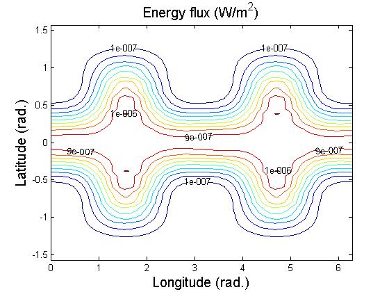
1. LTE_linear.f solves the Laplace tidal equations with (linear) Rayleigh dissipation. If run without changes, this program produces the plots seen in Figure 4 of the article, but users can easily modify it to solve many other linear tidal dissipation problems. The default output consists of surface plots of U,V and η at 0%,25%,50%,75%,100% of the way through the last period, and two plots with the time-averaged geographical distribution of the tidal dissipation rate.

2. LTE_nonlinear.f solves the Laplace tidal equations with (nonlinear) bottom drag. If run without changes, this program produces the result seen in line 1 of Table 2 of the article and if 'mode' is changed to 2, it produces the result of line 1 of Table 3, but users can easily modify it to solve many other nonlinear tidal dissipation problems. The default output consists of surface plots of U,V and η at 0%,25%,50%,75%,100% of the way through the last period, and two plots with the time-averaged geographical distribution of the tidal dissipation rate.

3. LTEice_linear.f solves the Laplace tidal equations with (linear) Rayleigh dissipation, including the effects of an ice cap. If run without changes, this program produces the plots seen in Figure 7 of the article, but users can easily modify it to solve many other linear tidal dissipation problems, with ice cap. The default output consists of surface plots of U,V, η and Q at 0%,25%,50%,75%,100% of the way through the last period, and two plots with the time-averaged geographical distribution of the tidal dissipation rate.

4. LTEice_nonlinear.f solves the Laplace tidal equations with (nonlinear) bottom drag, including the effects of an ice cap. If run without changes, this program produces the result for ocean depth = 100m in Figure 8a of the article, but users can easily modify it to solve many other nonlinear tidal dissipation problems, with ice cap. The default output consists of surface plots of U,V, η and Q at 0%,25%,50%,75%,100% of the way through the last period, and two plots with the time-averaged geographical distribution of the tidal dissipation rate.