Molecular Dynamics Simulation (MDSim) Module
I. Introduction to Molecular Mechanics
Molecular modeling defines intermolecular interactions in mathematical terms in an effort to predict and mimic behavior of molecular systems. Computational techniques have revolutionized this field of molecular mechanics and made calculations and predictions easier, especially with the help of high-performance computers in recent studies. The application of this molecular modeling in bioinformatics has led to a better understanding of movements and interactions of macromolecules.
Macromolecules are treated as a composite entity made up of elemental units, the atoms. In elemental chemistry, atom is made up of electrons, protons, and neutrons. Molecules are formed by atomic bonds that are formed by sharing of electrons. Atoms and molecules need to be specifically given positional coordinates in order to place them at the correct angle and orientation in a molecular modeling software program. There are represented by the Cartesian coordinate system, or alternatively by internal coordinate system represented by Z-matrix.
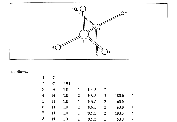
A. Z-Matrix Representation of Ethane
Figure 1: Staggered conformation of ethane
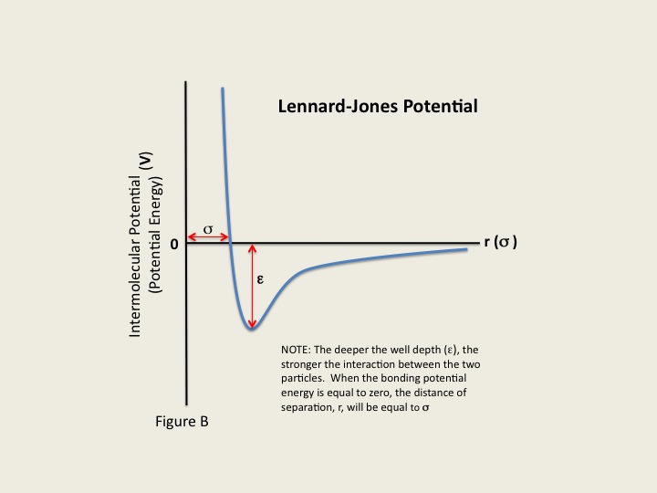
The energy of a molecule can be considered a function of the nuclear coordinates, which fluctuates due to the movement of its atoms and bonds resulting in the deviation of the bond lengths from the optimal values. At 3 kcal/mol, for example, a covalent bond between carbon atoms can be disrupted, with changes in the bond angles and torsional angles of the atoms. A function of the nuclear coordinates gives the energy of the molecule, which is termed as the Lennard-Jones Potential Energy (also referred to as the L-J potential, 6-12 potential, or 12-6 potential), a mathematically simple model that approximates the interaction between a pair of neutral atoms or molecules. The Lennard-Jones Potential (V) is the intermolecular potential given by :
where ϵ is the well depth and a measure of how strongly the two particles attract each other. σ is the distance at which the intermolecular potential between the two particles is zero. σ gives a measurement of how close two nonbonding particles can get and is thus referred to as the van der Waals radius. It is equal to one-half of the internuclear distance between nonbonding particles. And lastly, r is the distance of separation between both particles (measured from the center of one particle to the center of the other particle).
Figure 2: Lennard-Jones Potential, epsilon, and sigma [3]
Equation describes both the attractions and repulsions between nonionic particles. The first part of the equation, (σ/r)12 describes the repulsive forces between particles while the latter part of the equation, (σ/r)6 denotes attraction.
B. Bonding Potential
As mentioned earlier, the Lennard-Jones Potential is a function of the distance between the centers of two particles. When two nonbonding particles are an infinite distance apart, the possibility of them coming together and interacting is minimal. For the sake of simplicity then, we can say that their bonding potential energy is zero. However, as the distance of separation decreases, the probability of interaction increases. The particles come closer together until they reach a region of separation where the two particles become bound and their bonding potential energy decreases from zero to become a negative quantity. While the particles are bound, the distance between their centers will continue to decrease until the particles reach an equilibrium, which is specified by the separation distance at which the minimum potential energy is reached. Now, if we keep pushing the two bound particles together passed their equilibrium distance, repulsion begins to occur, as particles are so close to each other that their electrons are forced to occupy each other’s orbitals. Therefore, repulsion occurs as each particle attempts to retain the space in their respective orbitals. Despite the repulsive force between both particles, their bonding potential energy rises rapidly as the distance of separation between them decreases below the equilibrium distance.
C. Stability and Force of Interactions
Stability and Force of Interactions Very much like the bonding potential energy, the stability of an arrangement of atoms is also a function of the Lennard-Jones separation distance. As the separation distance decreases below equilibrium the potential energy becomes increasingly positive (force is repulsive). Such a large potential energy is energetically unfavorable as it indicates an overlapping of atomic orbitals. However, at long separation distances, the potential energy is negative and approaches zero as the separation distance increases to infinity (force is attractive). This indicates that at such long-range distances, the pair of atoms or molecules experiences a small stabilizing force. Lastly, as the separation between the two particles reaches a distance slightly greater than σ, the potential energy reaches a minimum value (force is zero). At this point, the pair of particles are most stable and will remain in that orientation until an external force is exerted upon them.
Figure 3: Lennard-Jones Potential, equilibrium distance, and forces [3]
These energy functions are optimum to certain set of coordinates. Once they are not in their optimum lengths and specifications the energy space is infinite to find the local minima and global minima. In order to reduce the search space, there are allowed range of angles and bond lengths and other parameters specified. The collection of these parameters are called Force Fields. So when a molecular system is in a particular force field, the molecule is restrained to the parameters specified in the force field. This force fields are highly employed during MDSim to avoid blind search for local minima and a stable configuration of the macro molecule.
II. Energy Minimization
A. Introduction
For all except a simple molecular configuration the energy calculations are complicated and are made of multidimensional function of the coordinates. The way in which the energy varies with the coordinates is usually referred to as the potential energy surface or the hyper surface. In molecular modeling we are specifically interested in the minimum points in this energy surface. Minimum energy configuration corresponds to the stable state of the system. In computational chemistry, energy minimization is also called geometry minimization which is used to compute the equilibrium configuration of molecules and solids. Stable states of molecular systems correspond to global and local minima on their potential energy surface. Starting from a non-equilibrium molecular geometry, energy minimization employs the mathematical procedure of optimization to move atoms so as to reduce the net forces (the gradients of potential energy) on the atoms until they become negligible.
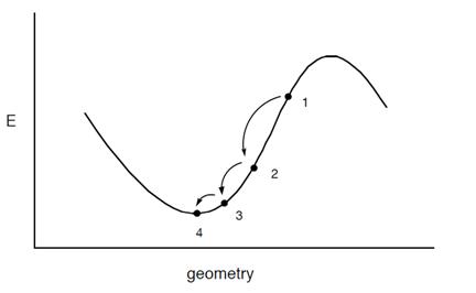
Like MD and Monte-Carlo approaches, periodic boundary conditions have been allowed in energy minimization methods, to make small systems. A well-established algorithm of energy minimization can be an efficient tool for molecular structure optimization. Energy minimization is a numerical procedure for finding a minimum on the potential energy surface starting from a higher energy initial structure, labeled “1” as illustrated in figure 1. During energy minimization, the geometry is changed in a stepwise fashion so that the energy of the molecule is reduced from steps 2 to 3 to 4 as shown in the figure 1. After a number of steps, a local or global minimum on the potential energy surface is reached.
Figure 4: Stepwise changes in the molecule's geometry by energy minimization from point 1 to 4
Most energy minimization methods proceed by determining the energy and the slope of the function at point 1. If the slope is positive, it is an indication that the coordinate is too large (as for point 1). If the slope is negative, then the coordinate is too small. The numerical minimization technique then adjusts the coordinate; if the slope is positive, the value of the coordinate is reduced as shown by point 2. The energy and the slope are again calculated for point 2. If the slope is zero, a minimum has been reached. If the slope is still positive, then the coordinate is reduced further, as shown for point 3, until a minimum is obtained. There are numerous methods for actually varying the geometry to find the minimum; only a few will be discussed here. Many of the methods used to find a minimum on the potential energy surface of a molecule use an iterative formula to work in a step-wise fashion. These are all based on formulas of the type: xnew = xold + correction
In the equation, xnew refers to the value of the geometry at the next step (for example, moving from step 1 to 2 in the figure), xold refers to the geometry at the current step, and correction is some adjustment made to the geometry. In all these methods, a numerical test is applied to the new geometry (xnew) to decide if a minimum is reached. For example, the slope may be tested to see if it is zero within some numerical tolerance. If the criterion is not met, then the formula is applied again to make another change in the geometry.
B. Newton-Raphson Method
The Newton-Raphson method is the most computationally expensive per step of all the methods utilized to perform energy minimization. It is based on Taylor series expansion of the potential energy surface at the current geometry. The equation for updating the geometry is xnew = xold – [E'' (xold )/E'''' (xold )]Notice that the correction term depends on both the first derivative (also called the slope or gradient) of the potential energy surface at the current geometry and also on the second derivative (otherwise known as the curvature). It is the necessity of calculating these derivatives at each step that makes the method very expensive per step, especially for a multidimensional potential energy surface where there are many directions in which to calculate the gradients and curvatures. However, the Newton-Raphson method usually requires the fewest steps to reach the minimum.
C. Steepest Descent Method
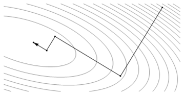
Rather than requiring the calculation of numerous second derivatives, the steepest descent method relies on an approximation. In this method, the second derivative is assumed to be a constant. Therefore, the equation to update the geometry becomes xnew = xold − γ E'' (xold )where, γ is a constant. In this method, the gradients at each point still must be calculated, but by not requiring second derivatives to be calculated, the method is much faster per step than the Newton-Raphson method. However, because of the approximation, it is not as efficient and so more steps are generally required to find the minimum. The method is named Steepest Descent because the direction in which the geometry is first minimized is opposite to the direction in which the gradient is largest (i.e., steepest) at the initial point. Once a minimum in the first direction is reached, a second minimization is carried out starting from that point and moving in the steepest remaining direction. This process continues until a minimum has been reached in all directions to within a sufficient tolerance.
Figure 5: Illustration of the Steepest Descent Method for a system with two geometrical coordinates
D. Conjugate Gradient Method
In the Conjugate Gradient method, the first portion of the search takes place opposite the direction of the largest gradient, just as in the Steepest Descent method. However, to avoid some of the oscillating back and forth that often plagues the steepest descent method as it moves toward the minimum, the conjugate gradient method mixes in a little of the previous direction in the next search. This allows the method to move rapidly to the minimum. These are the different energy minimization methods.
III. MDSim Methods
A. Introduction
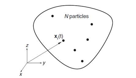
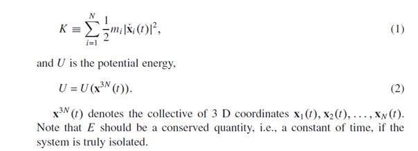
Macromolecules in our body are always in motion with changing configurations at different times for different functions. MD is an outcome of an immense research on molecular physics to understand particles in motion of a system. Its applications in biology have emerged when biophysics techniques involving experimental determination of biomolecular structures are being developed. A working definition of MDSim is technique by which one generates the atomic trajectories of a system of N particles by numerical integration of Newton’s equation of motion, for a specific interatomic potential, with certain initial condition (IC) and boundary condition (BC). Consider, for example (see Figure 6), a system with N atoms in a volume Ω. We can define its internal energy: E ≡ K +U, where K is the kinetic energy,
Figure 6: Illustration of the MDSim system
One can often treat an MDSim like an experiment. Below is a common flowchart of an ordinary MD run:
in which we fine-tune the system until it reaches the desired condition (here, temperature T and pressure P), and then perform property averages, for instance calculating the radial distribution function g(r) or thermal conductivity. One may also perform a non-equilibrium MD calculation, during which the system is subjected to perturbational or large external driving forces, and we analyze its non-equilibrium response, such as in many mechanical deformation simulations.
There are five key ingredients to an MD simulation, which are boundary condition, initial condition, force calculation, integrator/ensemble, and property calculation. A brief overview of them is given below, followed by more specific discussions. Boundary condition: There are two major types of boundary conditions: isolated boundary condition (IBC) and periodic boundary condition (PBC). IBC is ideally suited for studying clusters and molecules, while PBC is suited for studying bulk liquids and solids. Boundary condition are set to confine the motion of the molecules in the system.
Initial condition: Since Newton’s equations of motion are second-order ordinary differential equations (ODE), IC basically means x3N (t = 0) and x3N (t = 0), the initial particle positions and velocities. Generating the IC for crystalline solids is usually quite easy, but IC for liquids needs some work, and even more so for amorphous solids. A common strategy to create a proper liquid configuration is to melt a crystalline solid. And if one wants to obtain an amorphous configuration, a strategy is to quench the liquid during a MD run.
Force Calculation: Then Lennard Jones potential is calculated. For long-range Coulomb interactions, special algorithms exist to break them up into two contributions: a short-ranged interaction, plus a smooth, field-like interaction, both of which can be computed efficiently in separate ways.
Integrator/Ensemble: Different conformers are generated orderly and the conformation ensemble is integrated to get the virtual movie of the change in conformers of the molecule of the system.
Property calculation: A great value of MDSim is that it is “omnipotent” at the level of classical atoms. All properties that are well-posed in classical mechanics and statistical mechanics can in principle be computed.
IV. MD and Its Applications
A. Introduction
MD is a computational simulation method to understand the movement of particles in a system. The atoms and molecule interact with each other based on constraints and restraints posed on to the system. There are a variety of methods for studying molecules of interest in life sciences and related areas of chemistry. One of such methods is molecular mechanics/dynamics where atoms are treated as points with mass and charge, governed by the laws of classical physics. In MDSim, successive configurations of the system are generated by integrating Newton’s laws of motion. The result is a trajectory that specifies how the positions and velocities of the particles in the system vary with time. The main concept involved here is based on F=ma (newton’s law).
B. Background
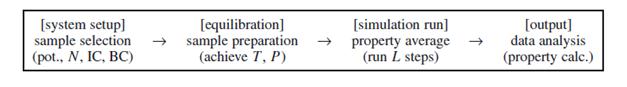
The first MDSim was performed in 1957 by Alder and Wainwright. In this model, the spheres move at a constant velocity in straight lines between collisions. All collisions are perfectly elastic and occur when the separation between the centers of spheres equals to the sphere diameter
The two main families of simulation technique are MD and Monte Carlo (MC); additionally, there is a whole range of hybrid techniques which combine features from both. The obvious advantage of MD over MC is that it gives a route to dynamical properties of the system: transport coefficients, time-dependent responses to perturbations, rheological properties and spectra.
Computer simulations act as a bridge between microscopic length and time scales and the macroscopic world of the laboratory: It provides a guess at the interactions between molecules, and obtain "exact" predictions of bulk properties. The predictions are "exact" in the sense that they can be made as accurate as we like, subject to the limitations imposed by our computer budget. At the same time, the hidden detail behind bulk measurements can be revealed. C: Applications There are 5 major applications of MDSim in Bioinformatics:
V. Setting Up a MDSim
A. Introduction
MD studies have been a key tool in understanding the dynamics, movements and interactions of proteins, lipids and other small molecules. It is a computer simulation of physical movements of atoms and molecules in a system or a specific environment. MD studies help us gain a deeper insight into the architecture of proteins and their movements inside our body. They have also become a common tool to investigate structure-activity relationships between macromolecules. Given their application in the field of protein biology, MDSim helps in simulating the experimental data to obtain information that cannot be experimentally obtained. For a macromolecule with 100,000 atoms, a simulation on a time scale of nanoseconds have become standard. B. Softwares used
There are multiple software which are being used by many scientific communities depending on their necessities and questions they wish to address using MDSim. Two major softwares used by them are 1) GROMACS [GROningen MAchine for Chemical Simulations] 2) NAMD [Not (just) Another MD program].
GROMACS is one the widely used MD software package. It is a MD package primarily designed for biomolecular systems such as proteins and lipids. It was originally developed in the Biophysical Chemistry department of University of Groningen, and is now maintained by contributors in universities and research centers across the world. GROMACS is one of the fastest and most popular software packages available and can run on CPUs as well as GPUs. It is free, open source released under the GNU General Public License. It can be downloaded from http://www.gromacs.org/Downloads. The software was written in C, C++ and assembly language
C. Setting Up Initial Configuration
First step while setting up a MDSim will be establishing an initial configuration of the system and the molecule (In this case, a macromolecule which is globular protein of interest). This initial configuration can be obtained either by experimental data which could be a structure that is experimentally determined by methods like X-ray crystallography, NMR or electron microscopy or by a predicted model using computation software involving molecular modeling techniques or by a combination of both. Once the initial structure or configuration of the protein is ready then MDSim is performed. D. Generating Topology Files
The first step in any software is to generate topology files. This topology file is ASCII coded and defines the entire topology of the system. The next step is to define the restraints to be imposed on the molecule. Some problems wants to address the entire movement of the protein or macromolecule while some wishes to address the movement of one particular domain. During the second case, the part which is not of interest or which wants to be static are restrained from movements. Another main step while setting up a MDSim is to define the proper force field in which the molecule is to be simulated. E. Setting up Water Box
MD studies has been a key tool in understanding the dynamics, movements and interactions of proteins, lipids and other small molecules. It is a computer simulation of physical movements of atoms and molecules in a system or a specific environment. MD studies help us gain a deeper insight into the architecture of proteins and their movements inside our body. They have also become a common tool to investigate structure-activity relationships between macromolecules. Given their application in the field of protein biology, MDSim helps in simulating the experimental data to obtain information that cannot be experimentally obtained. For a macromolecule with 100,000 atoms, a simulation on a time scale of nanoseconds have become standard. F. Adding Ions
The next step is to neutralize the charge in the system. Proteins in a solvent system carry charge. To neutralize the charge, Sodium ions are added to neutralize the excess negative charge carried in the system. G. Energy Minimization:
The major step is the next one where the system is energy minimized. Energy minimization is a key step to finding a configuration which stable and minimized locally from which the search space for the protein movement starts. The solvated, electro neutral system is assembled. Before beginning dynamics, Energy minimization ensures that the system has no steric clashes or inappropriate geometry. The structure is relaxed during this process. H. Equilibration:
EM ensures a reasonable starting structure, in terms of geometry and solvent orientation. To begin real dynamics, equilibrating the solvent and ions around the protein is mandatory. If one were to attempt unrestrained dynamics at this point, the system may collapse. The reason is that the solvent is mostly optimized within itself, and not necessarily with the solute. It needs to be brought to the temperature the system is wished to simulated and establish the proper orientation about the solute (the protein). After arriving at the correct temperature (based on kinetic energies), pressure is applied to the system until it reaches the proper density. During solvation the restrain files generated earlier will be involved. Movement is permitted, but only after overcoming a substantial energy penalty. The utility of position restraints is that they allow the system to equilibrate the solvent around the protein, without the added variable of structural changes in the protein.
Equilibration is often conducted in two phases. The first phase is conducted under an NVT ensemble (constant Number of particles, Volume, and Temperature). This ensemble is also referred to as "isothermal-isochoric" or "canonical." The timeframe for such a procedure is dependent upon the contents of the system, but in NVT, the temperature of the system should reach a plateau at the desired value. Next step is to stabilize the pressure (and thus also the density) of the system. Equilibration of pressure is conducted under an NPT ensemble, wherein the Number of particles, Pressure, and Temperature are all constant. The ensemble is also called the "isothermal-isobaric" ensemble, and most closely resembles experimental conditions. I. MD Run:
Upon completion of the two equilibration phases, the system is now well-equilibrated at the desired temperature and pressure. The position restraints are set and the MDSim is run for data collection. J. Results Analysis:
Now that the protein is simulated, the data of the position of the protein at every time step should be analyzed. The result analysis includes finding the movement of the protein, the RMSD calculation, Radius of Gyration calculation, etc. The results analysis depends on the biological question that is being asked which needed the MDSim.
VI. Case Study 1
Structural Rearrangement of Paramyxovirus F Protein During Membrane Fusion:
This case study clearly portrays the applications of MD in the field of biology and how efficient tool is it in understanding the protein process and function. The fusion of paramyxovirus to the cell membrane is mediated by fusion protein (F protein) present in the virus envelope, which undergoes a dramatic conformational change during the process.
The trimeric domain was simulated conformational change of the HRA region of F protein is produced during the first steps of the fusion of viral and cell membranes in paramyxoviruses. The model suggests that the cause of the reorganization could be a mechanical force that elongates the HRA segment, followed by relaxation and refolding of the region into an all-alpha state. Conformational change of F protein was simulated by steered MD procedures, using the SANDER module of the AMBER 10 package. The steered MD process started with the adaptation of the initial structure to the AMBER force field through 5000 steps of energy minimization, using the conjugate gradient method combined with four initial steps of steepest descent in each iteration. This minimization was performed with no restrictions added to the initial structure. The system was then heated over 10,000 steps of equilibration, which raised the temperature from 0 to 300 K, while restraining the position of the Ca atoms. Finally, torsion restrictions were removed from the segment spanning residues in order to start the MD. The Ramachandran plots verifies the structural integrity of the structures.
This clearly explains the application of MD in understanding the conformational changes of proteins
VII. Case
Study 2
Transmembrane Protein Dynamics
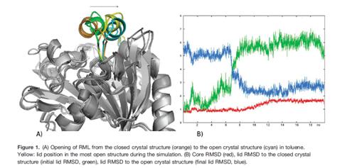
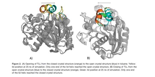
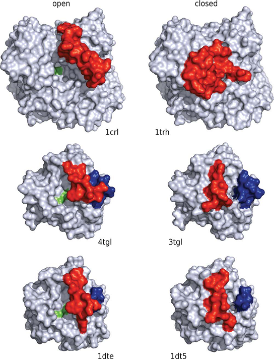
The second case study is about the application of MD in understanding the transmembrane protein movement. Most of the transporter proteins have two states. An active state and an inactive state. The protein is active when it readily performs its enzymatic function. When it is in an inactive form, it does not function. This state transition of the proteins is aided by structural change in the protein. For example in lipases. In most lipases, a mobile lid covers the substrate binding site. In this closed structure, the lipase is assumed to be inactive. Upon activation of the lipase by contact with a hydrophobic solvent or at a hydrophobic interface, the lid opens. In its open structure, the substrate binding site is accessible and the lipase is active. Sascha Rehm et al deciphered the lid movement in three eukaryotic lipases. The molecular mechanism of this interfacial activation was studied for three lipases (from Candida rugosa, Rhizomucor miehei, and Thermomyces lanuginosa) by multiple MD simulations for 25 ns without applying restraints or external forces. As initial structures of the simulations, the closed and open structures of the lipases were used. Both the closed and the open structure were simulated in water and in an organic solvent, toluene. In simulations of the closed lipases in water, no conformational transition was observed. However, in three independent simulations of the closed lipases in toluene the lid gradually opened.
Thus, pathways of the conformational transitions were investigated and possible kinetic bottlenecks were suggested. The open structures in toluene were stable, but in water the lid of all three lipases moved towards the closed structure and partially unfolded.
Thus, in all three lipases opening and closing was driven by the solvent and independent of a bound substrate molecule.
VIII. References
| ||||||||||||||||||||||||||