
Protein-Protein Docking Using Bioinformatics Tools (PPDock) Module
I. Introduction
As cancerous cells and normal cells exhibit a few biochemical differences, many anticancer drugs affect normal rapidly growing cells in the intestine and bone marrow areas and hence are toxic. Capabilities to determine drug-target binding affinities to achieve high levels of selective drug actions on cancer cells would be very useful for designing anti-cancer therapeutics. Since the over expression of the Janus Kinase 3 (JAK-3) has been implicated in cancerous disorders like adult T-cell lymphoma/leukemia (ATLL), JAK-3 inhibition is expected to play a vital role in treatment of cancer. The objective of this project is to use docking studies to identify potential JAK-3 inhibitors from a number of putative substrates, namely anaplastic lymphoma kinase (ALK), Gene transcription factor II-I (TFII-I) etc. Let us start the process by taking ALK as a potential inhibitor. Follow the following steps to get the process done.
II. Step 1: Gathering Protein Data Bank (PDB) Files
PDB files are the collection of experimentally determined three-dimensional structures of macromolecules, which are generally used by researchers and students. The collection includes the atomic coordinates, crystallographic structure factors and NMR experimental data. It also includes name of molecules, primary and secondary structure information, ligand and biological assembly information, details about data collection and bibliographic citations.
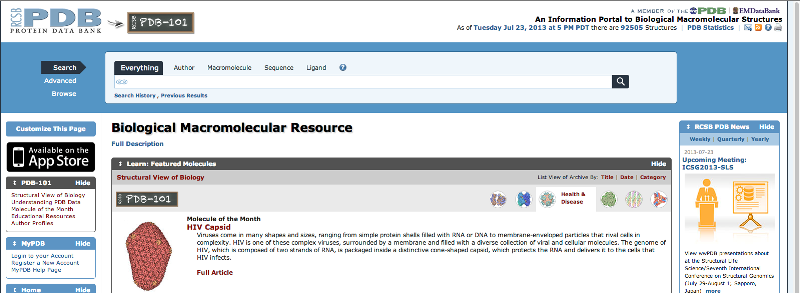
PDB files can be found at the following website: http://www.rcsb.org/pdb/home/home.do
Enter the PDB ID in the search bar as shown below
Figure
1: Screen shot of the RCSB PDB home page with the search bar included in it.
Gather the crystal structures of Jak3 and ALK (anaplastic lymphoma receptor tyrosine kinase) from RCSB Protein Data Bank. The crystal structures are available in PDB format. The pdb file of Jak3 is 1YVJ. The pdb file of ALK is 4DCE.
III. Step 2: Splitting PDB Files Using DECOMP
DECOMP is a web-based decomposition tool for splitting PDB files. Protein information technology group of Eotvos University located in Hungary developed it.
With this program, protein-ligand complexes can be identified reliably and the
ligands are deposited in separate files. Missing residues and atoms in chains
are handled properly and are inserted into chains for missing residues/atoms. DECOMP
server can be found at the following website: http://decomp.pitgroup.org/
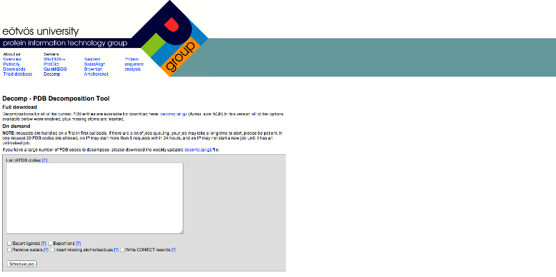
Figure
2: Screen shot of DECOMP server home page
Enter the PDB ID in the
empty box shown in the Figure 2. The pdb files of the
above two proteins are available along with their ligands. So we have to remove
the ligand. 1YVJ is the Jak3 kinase domain in complex with a straurosporine analogue. So we have to separate the straurosporine from the Jak3 kinase domain. In the same way
4DCE is anaplastic lymphoma kinase in complex with a piperidine-
carboxamide inhibitor. So we have to remove the
inhibitor.
Working with DECOMP:
We have to submit the pdb files of the proteins into the server. We are provided with various options to
export ligands, ions, and water molecules or to insert missing atoms or
residues. Choose the option to export ligand and submitted the files. The
requests are in the form of a queue i.e., first in first out and the time of
output depends on the traffic in the server. The output will be in the form of
a tar.gz files i.e. the compressed version. So after we extract the files from
the tar.gz files we have one directory for each of the pdb’s
listed. Each of these directories contains an error log with “.Error” extension
the decomposed pdb file with “.pdb”
extension and separate files of ligands or ions are present if the option
export ligand or ion was chosen.
From this directory take the decomposed pdb file i.e., a file with “.pdb” extension.
IV. Step 3: Use GRAMM to Predict the Interactions.
GRAMM (Global Range Molecular Matching) is a program
for protein docking. GRAMM is open source software and can be installed on the
personal computer. It is developed by the Vakser’s
lab (Center for Bioinformatics) belonging to university of Kansas. It can be
installed on MAC, Windows and Linux operating systems. The working instructions
given in this guide pertain to the windows version. It can be downloaded from
the following website. Its installation instruction was also given on the same
page.
http://vakser.bioinformatics.ku.edu/main/resources_gramm1.03.php
Working with GRAMM:
GRAMM has 3 parameter files rpar.gr, rmol.gr and
wlist.gr files. All these files are text files. I prefer using notepad to edit
these files.
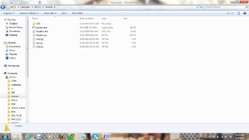
Figure
3: Screen shot of Gramm directory with its parameter files.
1) Parameters to be
considered for rpar.gr file:
The parameters for this file should be considered
based on the type of molecules we work with. The options available are
high resolution generic docking and low resolution generic docking. Let’s
try low-resolution generic docking in this case as we are not sure about the
structures of the given molecules and the parameters given for the low
resolution generic docking are:
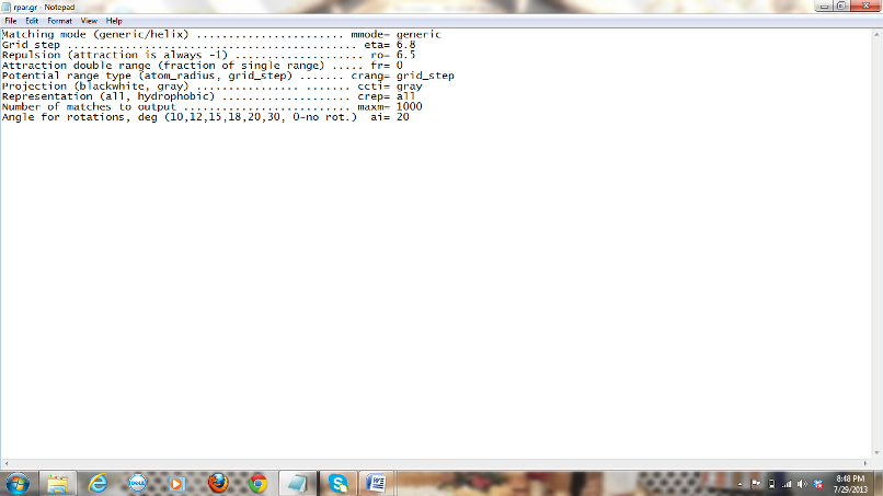
Figure 4: Screen shot of rpar.gr
file with the low generic docking parameters included.
2) The other file is
rmol.gr file. The following is the format of the file with the values I have
used:
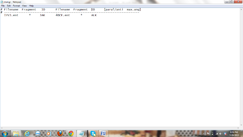
Figure 5: Screen
shot of rmol.gr file with parameters of JAK and ALK molecules included.
The two molecules to
which we need to see the predictions should be given here. Under the file name
we should give the name of one of the files with atomic coordinates (PDB
format). It should be converted in to .ent form before giving it here (1YVJ.ent). To change the
file format go to command prompt in windows. To open command prompt press
windows symbol on keyboard and type “cmd” in the
search bar and then press enter. A black screen appears on your desktop, which
is command prompt in windows. Now type the following commands in the command
prompt to rename the files.
C:\ Users\Name> cd C:\ (This command takes you to
C drive).
C:\>
cd Gramm (This command takes you to Gramm directory in C drive).
C:\Gramm> rename 1YVJ.pdb 1YVJ.ent (This command
renames the file)
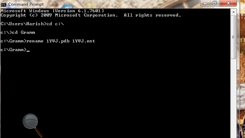
Figure
6: Screen shot of the command prompt after running Gramm to rename the PDB
files.
Under the column of the
fragment you have to mention the range of atoms for which the interactions are
to be found or simply you can give it as ’*’ so that the entire molecule can be
considered. Under the column of the ID you can give some string of characters
without spaces between them to identify your molecules. These ID’S will be used
by GRAMM to name the output files.
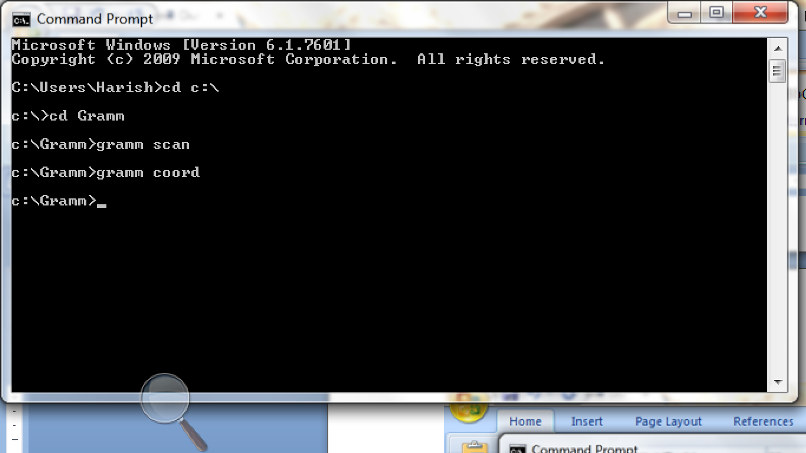
Run GRAMM with
parameter scan (gramm scan) from the terminal in the
GRAMM directory i.e., type “gramm scan” command in the
command prompt and press enter. It creates a .log file and .res file. To be
aware which grid has been chosen, see the output .log file. Grid is the
potential docking area in which the docking protein searches so as to release
maximum amount of energy up on reacting with the docked protein.
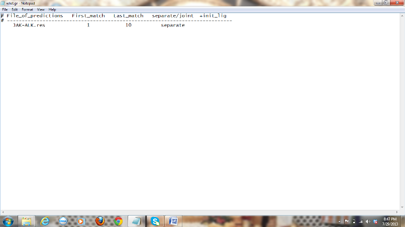
3) The last step is
giving parameters in wlist.gr file: The following is the format of the file
with the values I have used:
.res is the file that is obtained in the step b.
Figure
7: Screen shot of wlist.gr file with parameters included.
First match and last
match here refer to the retrieval of the top 10 hits from thousands of
complexes generated by Gramm. “Separate” here results in 10 separate pdb files instead of all the ten conformations in the same
file. If you want all the 10 conformations in the same pdb
file use “joint” Now run GRAMM with the parameter coord
(gramm coord) from the commands
prompt in the GRAMM directory i.e. type the command gramm
coord in the command prompt and press enter. Place
the GRAMM directory in C drive while you install.
C:\ Users\Name> cd C:\ (This command takes you to
C drive).
C:\>
cd Gramm (This command takes you to Gramm directory in C drive).
C:\ Gramm>gramm scan
(Creates .res and .log file).
C:\Gramm>gramm coord (Creates
the pdb files)
Figure
8: Screen shot of the command prompt after running gramm
scan and gramm coord
After
this you will finally get a file in .pdb format if
you use “joint” option in wlist.gr file or 10 separate pdb
files for this example if you use “seperate” option,
which shows us the various ways that the given two proteins interact.
V. Step 4: Visualizing Protein Interactions
Three tools that can
be used to visualize the final PDF files obtained from GRAMM are:
1) UCSF Chimera: It is a program for interactive
visualization and analysis of molecular structures. High quality images and
animations can be generated. It is developed by Resource for Biocomputing, Visualization
and Informatics (RBVI) Department belonging to University of California, San
Francisco. Download at http://www.cgl.ucsf.edu/chimera/download.html.
It can be used on windows, linux and Mac operating
systems.
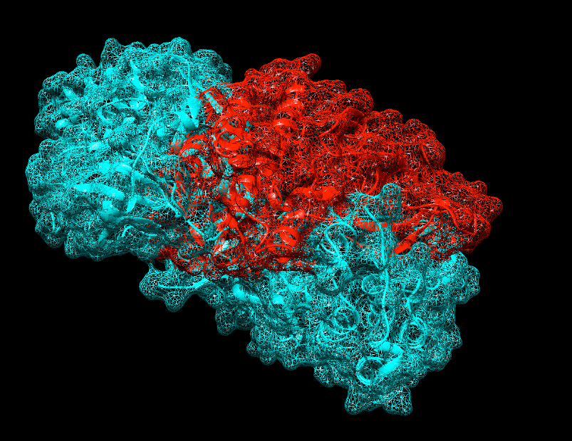
Figure
9: Screen shot showing JAK (Blue)-ALK (Red) complex in UCSF Chimera
2) Python Molecular viewer (PMV): PMV is a powerful
molecular viewer that has a number of customizable features. It is distributed
as a part of MGLTools, we need to download and
install MGLTools to get PMV. It is developed by Molecular Graphics
Laboratory of The Scripps Research Institute located in La Jolla, California. It
is freely available for download at http://mgltools.scripps.edu/.
It can be used on windows, linux and Mac operating
systems.
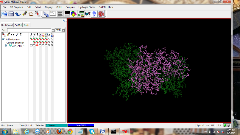
Figure
10: Screen shot showing JAK (Green)-ALK (Magenta) complex in PMV
3) Swiss-Pdb viewer: Swiss Pdb viewer can load and display several molecules
simultaneously. Each molecule is loaded into its own layer. It was developed by
The SIB Swiss Institute of Bioinformatics located in Switzerland. It is freely
available for download at http://spdbv.vital-it.ch/disclaim.html.
It can be used on windows, linux and Mac operating
systems.
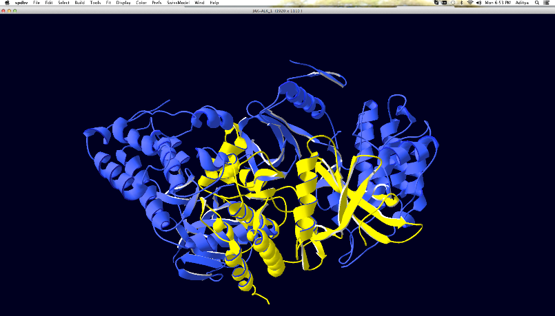
Figure
11: Screen shot showing JAK (Blue)-ALK (Yellow) complex in SPDBV Viewer
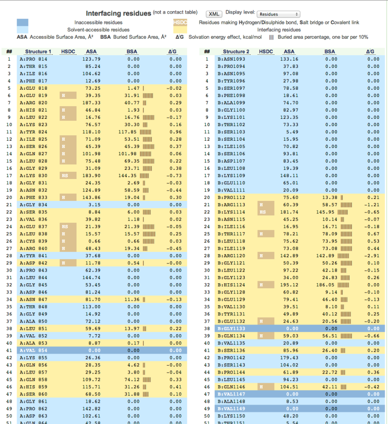
VI. Step 5: Showing Interfacial Amino Acids
Using servers such as SPPIDER and PISA server to get
to know about the interfacial amino acids, number of hydrogen bonds, interfacial
area and the amount of energy released. PISA server can be accessed at http://www.ebi.ac.uk/msd-srv/prot_int/.
SPPIDER can be accessed at http://sppider.cchmc.org/.
Some sample outputs are shown below:
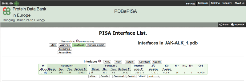
Figure
12: Screen of PISA server showing interfacial area, hydrogen bonds and the
Gibbs free energy

Figure
13: Screen shot about the atoms participating in
hydrogen bonds and salt bridges.
Figure
14: Screen shot showing detailed information about every atom of the complex
Continue this process
by taking other assumed potential inhibitors of Jak3. The molecule, which
releases highest amount of energy with Jak3, is considered the best inhibitor.
VII. References
Rosado, D.C. (2012) JAK3/STAT5 signalling cascade represents a therapeutic target to treat
select hematologic malignancies. ETD Collection for The University of Texas at El Paso, Paper AAI1512597.
Kontzias, A., Kotlyar, A.,
Laurence, A., Changelian, P., and O’Shea, J.J. (2012) Jakinibs: A New Class of Kinase Inhibitors in Cancer and
Autoimmune Disease. Curr. Opin. Pharmacol. 12(4):464-470. doi:10.1016/j.coph.2012.06.008.
http://www.ncbi.nlm. nih.gov/pmc/articles/PMC3419278. Accessed September 6, 2014.
Ordog, R., Szabadka, Z., and Grolmusz, V. (2009) DECOMP: APDB
decomposition tool on the web. Bioinformation 3(10):413-414. http://www.ncbi.nlm.nih.gov/pmc/articles/PMC2737496.