Protein Secondary Structure Analysis (PSSA) Module
I. IntroductionProteins are biochemical compounds consisting of one or more polypeptides typically folded into a globular or fibrous form in a biologically functional way. A polypeptide is a single linear polymer chain of amino acids bonded together by peptide bonds between the carboxyl and amino groups of adjacent amino acid residues. The sequence of amino acids in a protein is defined by the sequence of a gene, which is encoded in the genetic code. In general, the genetic code specifies 20 standard amino acids; however, in certain organisms the genetic code can include selenocysteine—and in certain archaea—pyrrolysine. Shortly after or even during synthesis, the residues in a protein are often chemically modified by posttranslational modification, which alters the physical and chemical properties, folding, stability, activity, and ultimately, the function of the proteins. Sometimes proteins have non-peptide groups attached, which can be called prosthetic groups or cofactors. Proteins can also work together to achieve a particular function, and they often associate to form stable protein complexes.
II. Levels of Protein Structure
A. Primary Structure
The primary structure refers to amino acid sequence of the polypeptide chain. Pimary structure is held together by covalent or peptide bonds, which are made during the process of protein biosynthesis or translation. The two ends of the polypeptide chain are referred to as the carboxyl terminus (C-terminus) and the amino terminus (N-terminus) based on the nature of the free group on each extremity. Counting of residues always starts at the N-terminal end (NH2-group), which is the end where the amino group is not involved in a peptide bond. The primary structure of a protein is determined by the gene corresponding to the protein. A specific sequence of nucleotides in DNA is transcribed into mRNA, which is read by the ribosome in a process called translation. The sequence of a protein is unique to that protein, and defines the structure and function of the protein. The sequence of a protein can be determined by methods such as Edman degradation or tandem mass spectrometry. Often however, it is read directly from the sequence of the gene using the genetic code. Post-translational modifications such as disulfide formation, phosphorylations and glycosylations are usually also considered a part of the primary structure, and cannot be read from the gene.
 Figure 1: Primary Structure (hypothetical) B. Secondary Structure (SS)
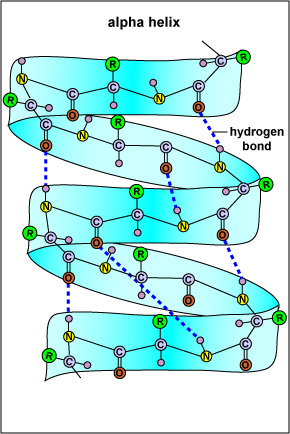
SS refers to highly regular local sub-structures. Two main types of SS, the alpha helix and the beta strand, were suggested in 1951 by Linus Pauling and coworkers. These SS are defined by patterns of hydrogen bonds between the main-chain peptide groups. They have a regular geometry, being constrained to specific values of the dihedral angles? and f on the Ramachandran plot. Both the alpha helix and the beta-sheet represent a way of saturating all the hydrogen bond donors and acceptors in the peptide backbone. Some parts of the protein are ordered but do not form any regular structures. They should not be confused with random coil, an unfolded polypeptide chain lacking any fixed three-dimensional structure. Several sequential SSs may form a "supersecondary unit".
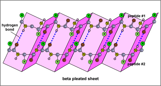 Figure 3: Beta-Pleated Sheet
The SS of a protein or polypeptide is due to hydrogen bonds forming between an oxygen atom of one amino acid and a nitrogen atom of another. There are two possible types of SS: an alpha helix and a beta sheet. In the case of an alpha helix, the hydrogen bonding causes the polypeptide to twist into a helix. With a beta sheet the hydrogen bonding enables the polypeptide to fold back and forth upon itself like a pleated sheet.
C. Tertiary Structure
Tertiary structure refers to three-dimensional structure of a single protein molecule. The alpha-helices and beta-sheets are folded into a compact globule. The folding is driven by the non-specific hydrophobic interactions (the burial of hydrophobic residues from water), but the structure is stable only when the parts of a protein domain are locked into place by specific tertiary interactions, such as salt bridges, hydrogen bonds, and the tight packing of side chains and disulfide bonds. The disulfide bonds are extremely rare in cytosolic proteins, since the cytosol is generally a reducing environment. ( In this module we will only deal with SSs)
D. Quaternary Structure
Quaternary structure is a larger assembly of several protein molecules or polypeptide chains, usually called subunits in this context. The quaternary structure is stabilized by the same non-covalent interactions and disulfide bonds as the tertiary structure. Complexes of two or more polypeptides (i.e. multiple subunits) are called multimers. Specifically it would be called a dimer if it contains two subunits, a trimer if it contains three subunits, and a tetramer if it contains four subunits. The subunits are frequently related to one another by symmetry operations, such as a 2-fold axis in a dimer. Multimers made up of identical subunits are referred to with a prefix of "homo-" (e.g. a homotetramer) and those made up of different subunits are referred to with a prefix of "hetero-" (e.g. a heterotetramer, such as the two alpha and two beta chains of hemoglobin). Many proteins do not have the quaternary structure and function as monomers.
III. Protein SS PredictionProtein SS helps in predicting 3D structure of proteins, and aid researchers in comprehending how proteins fold and interact with other molecules. This help us in developing new drugs by better understanding protein protein interactions. A. How to Predict SS? SS prediction is a set of techniques in bioinformatics that aim to predict the local SSs of proteins based only on knowledge of their primary structure — amino acid sequence, respectively. For proteins, a prediction consists of assigning regions of the amino acid sequence as likely alpha helices, beta strands (often noted as "extended" conformations), or turns. The success of a prediction is determined by comparing it to the results of the DSSP algorithm applied to the crystal structure of the protein; for nucleic acids, it may be determined from the hydrogen bonding pattern. Specialized algorithms have been developed for the detection of specific well-defined patterns such as transmembrane helices and coiled coils in proteins. Several algorithms are available as online servers. SS can be obtained by giving protein sequence in fasta format as input. B. SS Prediction Servers
In this module we will learn to predict SS using SS prediction servers when given a amino acid sequence. The SS can be evaluated by comparing them with the PDB structure. IV. Assignments
A. Assignment 1: Obtain 3KTS (Amino acid sequences are assigned with unique ID by PDB for easy access, 3KTS in this case) sequence from PDB. PDB is a protein data base containing 2D & 3D information. Type 3KTS in the PDB search box and click search. Information about PDB is avilable at http://en.wikipedia.org/wiki/Protein_Data_Bank. Click on "sequence" and download Fasta format of 3KTS protein sequence. In bioinformatics, FASTA format is a text-based format for representing either nucleotide sequences or peptide sequences, in which base pairs or amino acids are represented using single-letter codes. The format also allows for sequence names and comments to precede the sequences. The format originates from the FASTA software package, but has now become a standard in the field of Bioinformatics. Submit the FASTA sequence to SS prediction servers (links given above). Results will be mailed to provided mail id by the servers. Each server had a different way of sequence submission. All sequences should be given a identification short name (PDB ID can be used as short identifier). JPRED server predicts SS as you submite the protein sequece. (Make sure you dont close the webpage). All other servers mail their predictions to provided mail id. In some cases JUFO may not mail their predictions, you can access their predictions by clicking on results in the link below. Your submission can be identified from the identifier name you provided.
B. Assignment 2: Parsing using Perl
Results mailed to you by different SS prediction servers have lot of junk along with the SS predictions. We use Perl programming to parse all SS and the junk. Perl language provides powerful text processing facilities without the arbitrary data length limits of many contemporary Unix tools, facilitating easy manipulation of text files. Perl can be downloaded from link given below for free. Once installed all the Perl codes provided to you (with.pl extension) appears with an active Perl logo. Once Perl is installed you can parse the results mailed to you by the prediction servers. Name text files as given (in the example files).Once the results are mailed, Copy the results accordingly to the example files given into the text files. Each protein should have a separate folder with the Perl scripts and text files. All the text files and the Perl scripts should be saved in same folder. Perl scripts provided should be compiled in order. "Pars_servers" is compiled first to parse all the files obtained from different servers. "PDB_matrix" is compiled next to get matrix comparisons. "Matrix.pl" is compiled at the end to get overall comparision. Perl Download link: http://www.activestate.com/activeperl/downloads Perl scripts and example files: https://docs.google.com/document/d/1AniEw4oItJCFp1Pi8p8aDs6lneDE6z5NsfF637_Mb0w/edit?hl=en_US Save your identity percentages obtained from parsing scripts in a excel file. C. Assignment 3: Statistical analysis using R R is a programming language and software environment for statistical computing and graphics. The R language is widely used among statisticians for developing statistical software and data analysis. R uses a command line interface; however, several graphical user interfaces are available for use with R. R provides a wide variety of statistical and graphical techniques, including linear and nonlinear modeling, classical statistical tests, time-series analysis, classification, clustering, and others. R is easily extensible through functions and extensions, and the R community is noted for its active contributions in terms of packages. To make our work simple we use R studio. R studio is a free and open source integrated development environment (IDE) for R. You can run it on your desktop (Windows, MAc or Linux) or even over web using R studio Server. Download link: http://rstudio.org/. D. Assignment 4: Before we start, to get a basic idea on statistics and hypothesis testing please follow the links. Basic Statistics:
Hypothesis Testing: One-Way Repeated Measures ANOVA:
https://statistics.laerd.com/statistical-guides/repeated-measures-anova-statistical-guide.php In the one-way independent measures ANOVA, the total variability (SST) in data is divided into the between-group variability (SSB) and the within-group variability (SSW). In the one-way repeated measures ANOVA, we go one more step further and divide SSW into the subject variability (subject sum of squares, SSS) and the error variability (SSE). Hence, SST = SSB + SSS + SSE
The degrees of freedom associated with SSB, SSS, and SSE are (k-1), (N-1), and (k-1)*(N-1), respectively where k is the number of levels (servers, in our case), and N is the numbers of subjects (genes, in our case). The one-way repeated measures ANOVA, just like other ANOVAs, yields an F-statistic that is calculated as follows: F=(SSB/(k-1))/(SSE/[(k-1)*(n-1)]) Having introduced the one-way repeated measures ANOVA, in the following paragraphs, we will demonstrate how to conduct the one-way repeated measures ANOVA in R using the Anova(mod, idata, idesign) function from the car package. Tutorial Files Before we begin, you may want to download the sample data (.csv) used in this tutorial. Be sure to right-click and save the file to your R working directory. This dataset contains a sample of 30 genes whose expression is measured at three different cells using micro array analysis. The expression values are represented on a scale that ranges from 1 to 5 and indicate how different each gene is expressed in different cells. Data Setup Notice that our data are arranged differently for repeated measures ANOVA. In a typical one-way ANOVA, we would place all of the values of our independent variable in a single column and identify their respective levels with a second column, as demonstrated in this sample one-way dataset. In repeated measures ANOVA, we instead treat each level of our independent variable as if it were a variable, thus placing them side by side as columns. Hence, rather than having one vertical column for each cell, with a second column for expression levels, we have three separate columns for different cells, one for each cell. The following figure shows only first 5 rows of our data: Our hypothesis for this problem is R CODE Preparing the Repeated Measures Factor Step 1: Define the Levels 1. #use c() to create a vector containing the number of different cells within the repeated measures factor 2. #create a vector numbering the levels for our three different cells. 3. >differentcells <- c(1, 2, 3) Step 2: Define the Factor 1. #use as.factor() to create a factor using the level vector from step 1 2. #convert the differentcells into a factor 3. cellFactor <- as.factor(differentcells) Step 3: Define the Frame 1. #use data.frame() to create a data frame using the factor from step 2 2. #convert the cell factor into a data frame 3. cellFrame <- data.frame(cellFactor) Step 4: Bind the Columns 1. #use cbind() to bind the levels of the factor from the original dataset 2. #bind the cell columns 3. cellBind <- cbind(dataOneWayRepeatedMeasures$cell1, dataOneWayRepeatedMeasures$cell2, Step 5: Define the Model 1. #use lm() to generate a linear model using the bound factor levels from step 4 2. #generate a linear model using the bound cell levels 3. cellModel <- lm(cellBind ~ 1)
Loading the Anova(mod, idata, idesign) Function Conveniently, having already prepared our data, we can use a single Anova(mod, idata, idesign) function from the car package to yield all of the relevant repeated measures results. This allows us simplicity in that only a single function is required, regardless of the technique that we wish to employ. Thus, witnessing our outcomes becomes as simple as locating the desired method in the cleanly printed results. This function gives us several techniquies for analyzing repeated measures data, such as an epsilon-correction method, like Huynh-Feldt or Greenhouse-Geisser, or a multivariate method, like Wilks' Lambda or Hotelling's Trace. Our Anova(mod, idata, idesign) function will be composed of three arguments. First,mod will contain our linear model from Step 5 in the preceding section. Second, idatawill contain our data frame from Step 3. Third, idesign will contain our factor from Step 2, preceded by a tilde (~). Thus, our final function takes on the following form 1. #load the car package (install first, if necessary) 2. library(car) 3. #compose the Anova(mod, idata, idesign) function 4. analysis <- Anova(cellModel, idata = cellFrame, idesign = ~cellFactor) Visualizing the Results Finally, we can use the summary(object) function to visualize the results of our repeated measures ANOVA. 1. #use summary(object) to visualize the results of the repeated measures ANOVA 2. summary(analysis) Now with the identity percentages you obtained from using the parsing scripts. Analyze the data using the one way repeated ANOVA and make a decision if the means of the servers are equal or not. Quiz: Why do we use the One Way Repeated Measure ANOVA? What are µ1, µ2, & µ3 based on our obtained data? What is the null hypothesis for testing if the means of different servers are equal or not? What is the Alternative Hypothesis for testing if the means of different servers are equal or not? E. Assignment 5:
We use sample data (.csv) to learn this module. Make sure you download and save it in R working directory. This dataset contains a hypothetical sample of 30 participants who are divided into three stress reduction treatment groups (mental, physical, and medical). The values are represented on a scale that ranges from 1 to 5. This dataset can be conceptualized as a comparison between three stress treatment programs, one using mental methods, one using physical training, and one using medication. The values represent how effective the treatment programs were at reducing participant's stress levels, with higher numbers indicating higher effectiveness.
Assuming we have found a statistically significant difference among the mean effectiveness of treatments jointly, we naturally wonder from which treatment(s) this difference come(s). to investigate this, we would follow the one-way independent measures ANOVA by pairwise comparisons. We will use the Tukey's honestly significant difference (HSD) test to do the comparisons. One advantage of the test is that we keep the probability of finding a significant difference by chance in comparisons as a group at the significance level of the test. Hence, we can maintain the group-wise Type I error at the significance level of the test.
The Tukey's HSD test is very simple to perform. We first calculate HSD for each pairwise comparison and then compare it with the difference between the relevant two means. If the HSD is greater than the difference between the means, we reject the null hypothesis. HSD is calculated as follows: HSD=q* v(SSW/((N-k)*n)) , where n is the sample size for eash group, N is the total number of subjects, SSW is the within sum of squares from the one-way independent measures ANOVA, and q is the Studentized range statistic. Our Hypothesis for this problem is
After giving the basic idea about the Tukey's HSD test, we can now start hypothesis testing. Since we have three groups, we have. in fact, three pairwise comparisons. One of the hypotheses for our problem can be
H0: There is no honestly significant difference between µ1and µ2 H1: There is an honestly significant difference between µ1and µ2 Other hypotheses can be set similarly. Beginning Steps
To begin, we need to read our dataset into R and store its contents in a variable.
1. #read the dataset into an R variable using the read.csv(file) function
2.dataPairwiseComparisons <- read.csv("dataset_ANOVA_OneWayComparisons.csv")
3. #display the data
4. dataPairwiseComparisons
 The Tukey's HSD test can be executed using the TukeyHSD(x) function.
1. #HSD method
2. #use TukeyHSD(x), in tandem with aov(formula, data), to test the pairwise comparisons between the treatment group means
3. TukeyHSD(aov(StressReduction ~ Treatment, dataPairwiseComparisons))
Now with the identity percentages you obtained from using the parsing scripts. Analyze the data using the Tukey's HSD test scripts given and make a decision if the differences are honestly significant.
| ||||||||||||||||||||